Explaining the “Closing the ‘quantum supremacy’ gap” Paper
This is a translation of “Googleの量子超越性をスパコンで300秒で計算した論文を解説してみる” article.
The news that supercomputers have achieved to calculate Google's quantum supremacy demonstration task in 5 minutes was becoming hot news. This article explains the technical details and significance in the field of quantum computing.
BackgroundTensor NetworksBackground knowledgeOne-dimensional quantum stateTwo-dimensional quantum stateDependence of tensor network calculations performanceExample (ladder tensor)Order by a_1, a_2, a_4, a_3 Order by a_2, a_5, a_8, a_3Methodology of the 300-second paper on quantum supremacyOverviewMethodsOptimization of sum order by heuristicsResultsSummary and CommentsReferences
Background
In 2019, Google announced that “Sycamore,” a 53 qubits quantum computer that Google is developing, has achieved to solve a complex task that would (likely) take a tremendous amount of time with existing computers in 200 seconds.*1
Although this news got much attention, many groups, like IBM *2, replied that they could solve Google’s task practically using classical computers. Competition between quantum and existing computers was heating up.
In Oct. 2021, a paper stating that they finally finished the task in 300 seconds using supercomputers was published *3, and this topic has become hot again
Sadly, only the fact that “ Supercomputers has achieved to solve the task which indicates the quantum supremacy in 300 seconds“ comes up, and the technical details like how they achieved were never likely to be spoken. Therefor, I will explain it along with its background knowledge.
Tensor Networks
In this section, we discuss the overview of tensor networks and the benefits of this method.
Background knowledge
Quantum computation is a method of performing various operations on quantum states by applying operations called quantum gates. Many quantum circuits are illustrated in the figure below.

An example of quantum circuits
To simulate this process in an existing computer (also called a "classical computer" in contrast to a quantum computer), for example, when dealing with n qubits, we need the following vector wrepresentation for the quantum state
where the term
corresponds to the coefficients of the vector representing a quantum state, and since each takes a value , there are possible values takes. The classical computer has to manage all values, making the calculation fail even for relatively small values of .
Many kinds of research have been done to overcome this difficulty for a long time and have reached the conclusion that it is possible to improve and reduce the computational cost by dividing the coefficient into tensor products shown below
Today, this is known as tensor networks.
The following section will use this description to see how exactly a quantum circuit is represented.
One-dimensional quantum state
First, we consider the following qubits that are in a one-dimensional arrangement. Suppose that a two-qubit operation such as a CNOT gate acts only between qubits next to each other in this circuit.

The coefficients of the quantum state can then be represented using tensor network notation as follows,
where the schmatic diagram is illustrated as follows

In this diagram,
- White squares represent each tensor
- Lines coming from each tensor represent the index (like ) of the tensor
- If the same lines are joined, the inner product is computed for that index
Since summation of the inner product for an index removes that index from the equation, the last remaining index is the one that is left floating in the diagram with no lines joined. In the example above, these would be .
By changing the value of , which represents the range of the sum of , we can control the complexity of the quantum states.
For example, if we put 1 in , then coefficient would be
Since is just a scalar, it cannot represent correlations between qubits. Changing the value of allows us to represent correlations between different qubits. Since all qubits are not correlated (e.g., all ) at the beginning of the calculation, we start from .
Next, let us take this state and apply the following quantum gate which only affects
The result will be
Focusing only on the coefficients, we can convert them as below.
This shows that there is no effect on any other tensor except .
Therefor,we only need to rewrite the tensors which only affects as follows
And the coefficient of quantum state would be like this
Next, we will apply the two-qubit gate below that only affect and .
Applying this as before, we will get
Using singular value decomposition, this operator can be decomposed as follows
Re-substituting the coefficients again, and we will get
By using the equation below,
we can represent the quantum state after operation as follows.
Notice that and always appear together. By rewriting as , we can get the original notation.
The range of the sum of is because the degrees of freedom must also be taken into account. It can also be interpreted that the range of the sum of is expanded because the operations between the different qubits have led to correlations and complex quantum states.
In summary, the tensor network changes
- When applying a 1-qubit gate, the value of , the range of the sum of , does not change.
- When applying a 2-qubit gate, the value of , the range of sums of the corresponding indices ( in the example above), doubles.
The following is also a graphical representation of a 2-qubit gate in action. The thick line doubles the value of , indicating that the range of the sum of the index () between the first and second qubits has been expanded.

We can see how the value of increases by a factor of 2 as the depth of the circuit increases, making the calculation more difficult. *4
If the circuit is a random quantum circuit that acts on a gate between two qubits for every 8 depths, we can estimate as follows *5
Two-dimensional quantum state
We have discussed qubits arranged in one dimension, but this can be extended to the arrangement of qubits in general.
For example, if the qubits are arranged in two dimensions as shown below,

We can represent this as
The same can be said for applying 1-qubit gate and 2-qubit gate.
Dependence of tensor network calculations performance
Example (ladder tensor)
In order to obtain information about the calculated quantum state, we need to calculate the overlap of the two states. Please see here for specific calculation methods.
In this calculation, the order of summarizing can drastically change the calculation cost. As an extreme example, consider the following ladder-like tensor.

The equation can be written as follows (omitted hereafter).
Let us sum this tensor in two different ways.
Order by a_1, a_2, a_4, a_3
First, let's take the sum as we go from left to right. You will see that the tensor changes as follows.


In this case, we see that there are always only two lines that come out of the tensor generated in the course of the calculation. Therefore, the size of the tensor will not increase.
Order by a_2, a_5, a_8, a_3
Next, let’s take the sum as we go from top to bottom. The tensor changes as follows.


In this case, we can see that three or four lines come out of the tensor generated in the process of calculation. This represents an exponential enlargement of the tensor's size in the computation process.*6
In computing tensor network states, avoiding enlargement of the tensor size by choosing which sums to prioritize is essential to improve performance.
In this example, the order of summations to be taken can be determined at a glance, but for an arbitrary shape, the optimal order of summation evaluation is difficult to determine. For example, in the case of a 2-dimensional lattice model with , the sums must be taken either vertically or horizontally, and the exponential increase in tensor size by cannot be avoided. This is why the model used in Google's quantum transcendence is challenging to simulate on classical computers.
The problem of which sums of a tensor network should be prioritized to optimize computational cost is a difficult task in itself. Studies *7 have solved this problem using various heuristics *8. One of the tools used in this paper is a software called CoTenGra *9 , which was developed from this research.
Methodology of the 300-second paper on quantum supremacy
Finally, with all of this background knowledge in mind, we will discuss the paper written by Y. Liu, et al. (2021), computing the task used for quantum supremacy using a supercomputer in 300 seconds. it is certainly true that, they used massive numbers and the outstanding performance of supercomputers. However, even so, its performance cannot be fully utilized without appropriate parallelization, so we explain what kind of method they used.
Overview
In this research, calculations are performed using a large cluster on Sunway TaihuLight, a Chinese supercomputer, and the architecture diagram of each CPU is shown below.
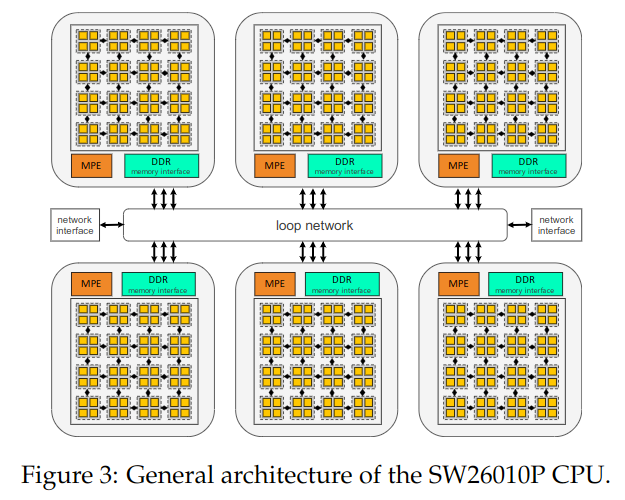
The system consists of 6 Core Groups in one CPU and 64 threads in each Core Group. In this research, 107,520 CPUs were used to simulate quantum circuits.
In order to simulate quantum circuits with such a large number of processes running in parallel, these are necessary.
- The task of taking the sum of the indices on the tensor network must be divided so that the above CPUs can be run in parallel without waste.
- Consider how to efficiently sum the indices not only for lattice-like qubits but also for arbitrary topology.
Methods
This paper simulated two circuits, a 10x10 lattice model of 100 qubits with (1+40+1)depth *10, i.e., 42 times of calculations, and the circuit ran on Google's Sycamore. Since they took different approaches to each of these two types of simulations, we discuss two techniques used to simulate circuits.
slicing
As mentioned earlier, the bottleneck in the computation of tensor networks was the growing size of tensors created as intermediate products when calculating the sum of tensor indices. However, there are cases where the computational cost could be greatly mitigated if the sum of some of the indices did not have to be computed.
Let us look at the ladder tensor network discussed above again.

If we do not need to take the sum of, say, of this index, then we can make the graph as follows.

And the formula will be
Note that no sum is taken for
In this case, we see that even if we compute the sum of the indices from top to bottom in order the tensor legs do not increase by more than because the network is disconnected at , unlike the previous example.
In other words, by fixing the possible values of , we can compute the sum of the tensor network indices for each value in parallel and add all the results later, so we can recover the original graph shape, reduce the computational difficulty of the tensor network, and even benefit from the parallelism of the supercomputer. This technique is called slicing. Essentially, they changed the spatial computational complexity into the sequential computational complexity and used the supercomputer superpower.
This method itself is not original to this paper but is also used in research published by IBM *11
In this paper's 10x10 lattice model of 100 qubits, slicing is performed in the following blue wavy line.

Assuming that the number of truncated indices (i.e., the number of non-summed indices) is 6 and that the range of the sum of the indices is about , then the depth is 40. It follows that roughly parallel computations are required, which is heavy work even at this point.
If you do slicing at this point, you can sum the tensor indices as follows. All rectangular in the below figures represent generated tensors


Summing in this order shows that the tensor connection is always kept at about 5 or 6, which reduces memory consumption by about , or about 30 million times, compared to dealing directly with the lattice model. The computation of the sum of each of these tensors is also parallelized.
Optimization of sum order by heuristics
While the above methods are applicable to lattice models, they may be inefficient for general models. In this study, they used software called CoTenGra *12 to calculate the appropriate slicing and summation order depending on the model geometry. The result is shown in the figure below.
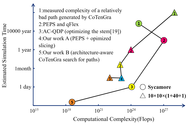
The markers 4 and 5 in the figure represent the lattice model with slicing and CoTenGra. The triangular plot shows the simulated results for the lattice model, and the circular plot shows the simulated results for Google's Sycamore model.
While CoTenGra does not change the performance of the lattice model, a significant performance improvement can be seen in Google's Sycamore model.
Other improvements
Almost all of the algorithms used are mentioned above, but other innovations are
- When calculating the sum of tensor indices, the elements to be calculated are extracted by DMA (Direct Memory Access) to optimize memory access, and then the tensor calculation is performed.
- Since there is a difference in the shape of the tensor when CoTenGra is used, a different method for optimization *13 is used to convert the tensor to a form that is easy to optimize. The conversion is performed in a form that is easy to optimize.
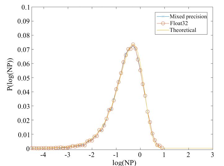
- Since single-precision floating-point (32-bit float variable) causes a bottleneck in calculation speed, after evaluating errors and confirming that there are no problems, calculations were performed using a mixture of half-precision floating-point (16-bit float) variables, and FLOPS were increased approximately 4 times (from 1.2Eflops to 4.4Eflops ).
Results
After these many efforts, the following figure shows that they were able to reproduce the Porter-Thomas distribution, which is the distribution that should be output by a random quantum circuit, and this paper claims that we were able to compute this distribution in 300 seconds.
Summary and Comments
The key points from the results of this paper are
- Proposed a method to compute in parallel on a supercomputer by converting the difficulty of spatial computational complexity into sequential computational complexity by slicing.
- Heuristics methods to compute efficient tensor summation order were introduced.
- Various other optimizations related to memory access were introduced.
My impression of this method is not that they have created a new method that changes everything, but rather that they combined existing methods in a very clever way and achieved an extraordinary performance. For example, in the tensor sum calculation, when calculating (1+40+1)depth with 10x10 qubits, the tensor size almost exceeds 16GB, the memory size of one Core Group, even when using single-precision floating decimals. This clearly indicates that the tensor size is crossing the edge of supercomputer specs. There may be many optimization techniques that are not explicitly mentioned in the paper. It is possible that this result could not have been achieved if the specs of the supercomputer had been a little lower, and I think it is too early to say that the quantum computer is useless just because the same task was solved in 300 seconds by a supercomputer.
On the other hand, I also feel that it would be interesting to see an UPDATE on the algorithm for classical computers. This paper is ultimately devoted to performing tensor calculations efficiently, but it has not been proven that tensor networks are the optimal method for representing quantum states *14. One possible way to outperform tensor network representation is to represent quantum states using Boltzmann machines *15.By combining such methods, it may be possible to create a much more efficient simulator on a classical computer.
I would like to conclude this paper's commentary with the hope that further methods will be developed.
References
*1: F. Arute, et al., Quantum supremacy using a programmable superconducting processor. Nature 574, 505–510 (2019)
*3: Y. Liu, et al., Closing the “Quantum Supremacy” Gap, Proceedings of the International Conference for High Performance Computing, Networking, Storage and Analysis (2021)
*4: Depending on the gate to be used, there may be a situation where no significant error is generated even if the sum of index () is not taken until the appropriate value and it is terminated. In such a case, for example, you can prepare a tensor network with smaller and optimize each coefficient parameter by the least-squares method, so that even if the depth increases, it can be easily handled by a classical computer, but in the case of a random quantum circuit like the one we are dealing with here, However, this should not be the case in the case of random quantum circuits such as the one we will be dealing with here.
*5: C. Guo, et al., General-Purpose Quantum Circuit Simulator with Projected Entangled-Pair States and the Quantum Supremacy Frontier, Phys. Rev. Lett. 123, (2019)
*6: For example, if each index takes 16 different values ( ), a 2-lined tensor would need to hold 16*16 = 256 elements, whereas a 10-legged tensor would have elements.
*7: J. Gray and S. Kourtis, Hyper-Optimized Tensor Network Contraction, Quantum 5, 410 (2021)
*8:Looking at this paper, it seems that one of the methods is to incorporate it into the community detection problem or to use meta-heuristics to select which sums to prioritize for calculation using the Boltzmann distribution.
*10: The reason why we dare to add 1 at the beginning and the end is to make the Adamar gate act on all qubits at the beginning and the end in the random quantum circuit scheme.
*11: E. Pednault, J. A Gunnels, G. Nannicini, L. Horesh, T. Magerlein, E. Solomonik, and R. Wisnieff. Breaking the 49-qubit barrier in the simulation of quantum circuits. arXiv preprint arXiv:1710.05867, 15, (2017)
*13: P. Springer and P. Bientinesi, Design of a High-Performance GEMM-like Tensor–Tensor Multiplication, ACM Trans. Math. Softw. 44, 1 (2018)
*14: For example, representing a cat state α|000> + β|111> with a tensor network framework requires large dimensions of the matrix, even though the state can be determined by only two coefficients α and β.
*15: Y. Nomura, A. S. Darmawan, Y. Yamaji, and M. Imada Phys. Rev. B 96, 205152 (2017)